Image

Tip

This requires Pillow and matplotlib dependencies. You can install them via pip install "docarray[full]"

Load image data

You can load image data by specifying the image URI and then convert it into .tensor using Document API

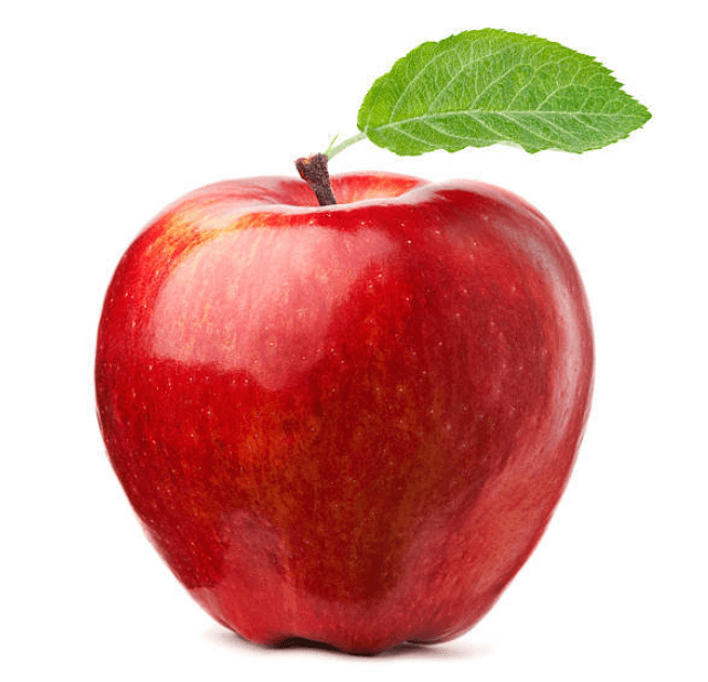
from docarray import Document

d = Document(uri='apple.png')
d.load_uri_to_image_tensor()

print(d.tensor, d.tensor.shape)

[[[255 255 255]
  [255 255 255]
  [255 255 255]
  ...
  [255 255 255]]]
(618, 641, 3)

DocArray also supports loading multi-page tiff files. In this case, the image tensors are stored to the .tensor attributes at the chunk-level instead of the top-level.

from docarray import Document

d = Document(uri='muti_page_tiff_file.tiff')
d.load_uri_to_image_tensor()

d.summary()

<Document ('id', 'uri', 'chunks') at 7f907d786d6c11ec840a1e008a366d49>
    └─ chunks
          ├─ <Document ('id', 'parent_id', 'granularity', 'tensor') at 7aa4c0ba66cf6c300b7f07fdcbc2fdc8>
          ├─ <Document ('id', 'parent_id', 'granularity', 'tensor') at bc94a3e3ca60352f2e4c9ab1b1bb9c22>
          └─ <Document ('id', 'parent_id', 'granularity', 'tensor') at 36fe0d1daf4442ad6461c619f8bb25b7>

Simple image processing

DocArray provides some functions to help you preprocess the image data. You can resize it (i.e. downsampling/upsampling) and normalize it; you can switch the channel axis of the .tensor to meet certain requirements of other framework; and finally you can chain all these preprocessing steps together in one line. For example, before feeding data into a Pytorch-based ResNet Executor, the image needs to be normalized and the color axis should be at first, not at the last. You can do this via:

from docarray import Document

d = (
    Document(uri='apple.png')
    .load_uri_to_image_tensor()
    .set_image_tensor_shape(shape=(224, 224))
    .set_image_tensor_normalization()
    .set_image_tensor_channel_axis(-1, 0)
)

print(d.tensor, d.tensor.shape)

[[[2.2489083 2.2489083 2.2489083 ... 2.2489083 2.2489083 2.2489083]
  [2.2489083 2.2489083 2.2489083 ... 2.2489083 2.2489083 2.2489083]
  [2.2489083 2.2489083 2.2489083 ... 2.2489083 2.2489083 2.2489083]
  ...
  [2.64      2.64      2.64      ... 2.64      2.64      2.64     ]
  [2.64      2.64      2.64      ... 2.64      2.64      2.64     ]
  [2.64      2.64      2.64      ... 2.64      2.64      2.64     ]]]
(3, 224, 224)

You can also dump .tensor back to a PNG image so that you can see.

d.save_image_tensor_to_file('apple-proc.png', channel_axis=0)

Note that the channel axis is now switched to 0 because the previous preprocessing steps we just conducted.

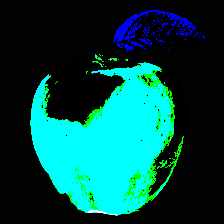
Yep, this looks uneatable. That’s often what you give to the deep learning algorithms.

Display image sprite

An image sprites is a collection of images put into a single image. When working with a DocumentArray of image Documents, you can directly view the image sprites via plot_image_sprites. This gives you a quick view of the dataset that you are working with:

from docarray import DocumentArray

da = DocumentArray.from_files('/Users/hanxiao/Downloads/left/*.jpg')
da.plot_image_sprites('sprite-img.png')

Depending on the number of images, this could take a while. But after that, you get a very nice overview of your DocumentArray as follows:

Segment large complicated image into small ones

A large complicated image is hard to search, as it may contain too many elements and interesting information and hence hard to define the search problem in the first place. Take the following image as an example,

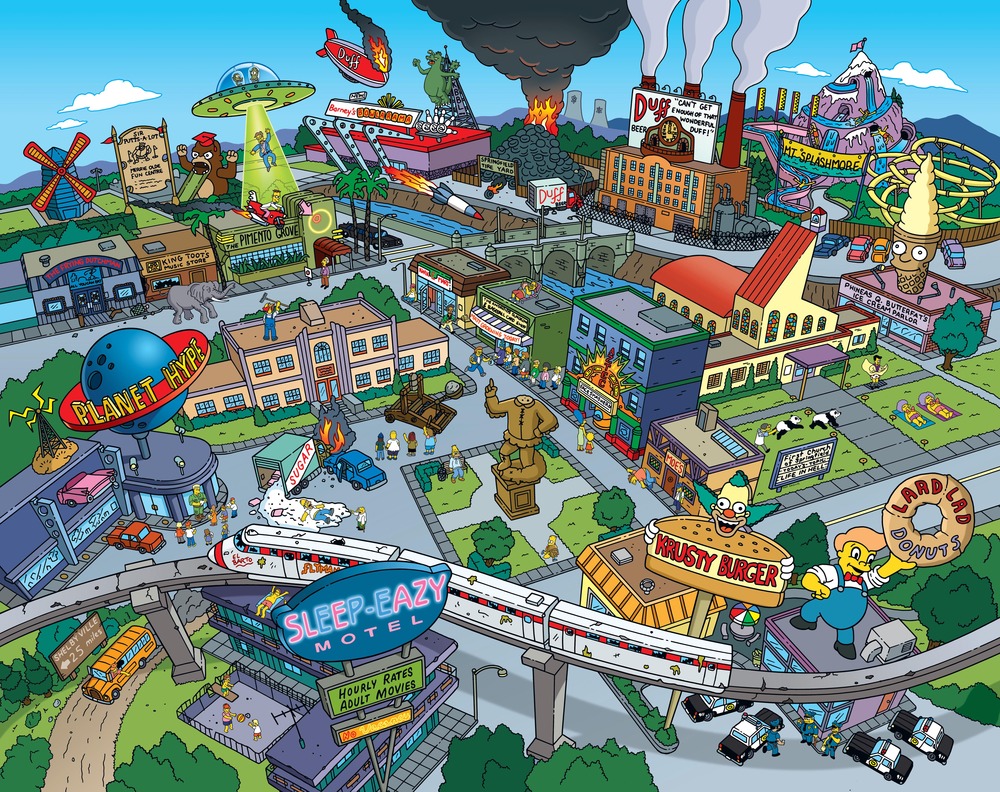
It contains rich information in details, and it is complicated as there is no single salience interest in the image. The user may want to hit this image by searching for “Krusty Burger” or “Yellow schoolbus”. User’s real intention is hard guess, which highly depends on the applications. But at least what we can do is using DocArray to breakdown this complicated image into simpler ones. One of the simplest approaches is to cut the image via sliding windows.

from docarray import Document

d = Document(uri='docs/datatype/image/complicated-image.jpeg')
d.load_uri_to_image_tensor()
print(d.tensor.shape)

d.convert_image_tensor_to_sliding_windows(window_shape=(64, 64))
print(d.tensor.shape)

(792, 1000, 3)
(180, 64, 64, 3)

As you can see, it converts the single image tensor into 180 image tensors, each with the size of (64, 64, 3). You can also add all 180 image tensors into the chunks of this Document, simply do:

d.convert_image_tensor_to_sliding_windows(window_shape=(64, 64), as_chunks=True)

print(d.chunks)

ChunkArray has 180 items (showing first three):
{'id': '7585b8aa-3826-11ec-bc1a-1e008a366d48', 'mime_type': 'image/jpeg', 'tensor': {'dense': {'buffer': 'H8T0H8T0H8T0H8T0H8T0H8T0H8T0H8T0H8T0H8T0H8T0H8T0H8T0H8T0H8T0H8T0H8T0H8T0H8T0H8T0H8T0H8T0H8T0H8T0H8T0H8T0 ...

Let’s now use image sprite to see how these chunks look like:

d.chunks.plot_image_sprites('simpsons-chunks.png')

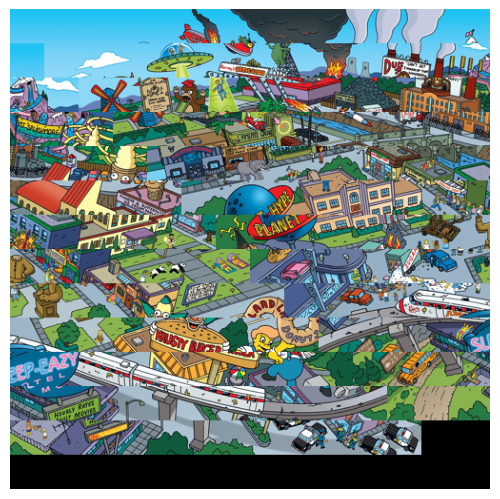
Hmm, doesn’t change so much. This is because we scan the whole image using sliding windows with no overlap (i.e. stride). Let’s do a bit oversampling:

d.convert_image_tensor_to_sliding_windows(
    window_shape=(64, 64), strides=(10, 10), as_chunks=True
)
d.chunks.plot_image_sprites('simpsons-chunks-stride-10.png')

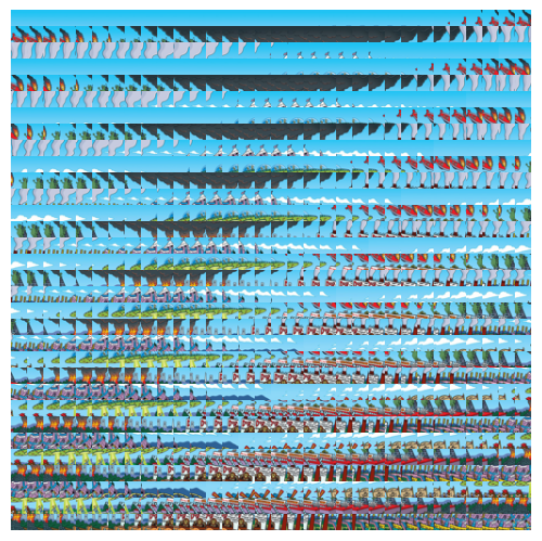
Yep, that definitely looks better.